저번시간에 합성곱으로 원과 네모를 구별하는 CNN을 어떻게 구성하고, 학습할 수 있는지 그림과 함께 알아보았다. 이번 시간에는 직접 코드를 작성해 보면서 가능한지 알아보자.
1. 준비하기
1) CNN 구성
Input → Conv2D → relu → Max Pooling → flatten → fc → sigmoid
2) 이미지 준비하기
아래의 파일을 다운받아 적절한 곳에 풀자.
28 × 28 이미지
train : 원 12개, 네모 12개
test : 원 2개, 네모 2개
3) train data
학습데이터를 불러오고 이미지를 출력해 보자.

이미지를 불러와서 Numpy 배열에 넣자. 주의할 점은 2가지가 있는데
(1) 흰색 바탕에 검은색 그림 → 반전(bitwise_not) 시켜 검은색 바탕에 흰색 그림으로 나타낸다. 왜냐하면 흰색 값이 크기 때문에 훈련에 도움이 되기 때문이다.
(2) 일반적으로 이미지 전처리 시 흑백 이미지(Grayscale)는 0 ~ 255.0 값을 가지고 있어 너무 크기 때문에 정규화를 하여 0 ~ 1 사이의 값을 가지게 한다. 이렇게 하면 relu 연산에서 아무것도 통과하지 못할 가능성이 크다! (relu 연산은 0보다 크면 통과하기 때문) 따라서 /255.0 정규화가 아닌 0 ~ 10사이의 값을 가지는 10/255로 정규화 하면 relu 연산에서 큰 문제를 일으키지 않는다.
→ 위 2가지 문제를 고려하지 않고 제시된 대로 신경망을 작동하면 어떻게 될까? 직접 해 보는 것도 나쁘지 않다.
이미지를 직접 불러와서 matplotlib를 이용해 그려보자. 동그라미와 네모가 참 개성 있으면서도 제각각 그려진 것을 알 수 있다.
4) test data
학습데이터를 불러오고 이미지를 출력해 보자.
5) 학습 목표(targets) 설정하기

원을 0, 네모를 1로 설정한다. np.repeat을 이용해 0 또는 1로 채우고 concatenate를 이용해 결합하여 (batch, target)으로 구성한다.
6) Hyper parameter 설정하기

가중치와 stride, padding, filter size, output size 등을 설정한다. 엡실론(epsilon)을 0.0001로 설정해 두었는데 sigmoid 함수 역전파 시 0으로 나누는 문제가 발생할 수 있고 이를 해결하기 위해 도입하였다.
참고 : 이진 교차 엔트로피 역전파시 0으로 나누는 에러 발생 해결방법, 엡실론 추가
2. 합성곱, 풀링 함수 작성하기
합성곱, 최대 풀링을 구현하기 위한 함수를 작성한다. 이전시간에 쭉 했던 내용이라 설명은 패스


3. 순전파 구현하기
forward 함수를 작성하여 순전파를 구현한다.
inputs = train_X (batch, 28, 28)임을 떠올려 연산 후 shape이 어떻게 변하는지 주석을 잘 보면서 관찰하자.
losses에서 np.log1p를 사용하였는데 sigmoid 출력이 0에 가깝게 되면 -∞ 문제가 발생하게 될 수 있다. 이를 방지하기 위해 범위를 0 ~ 1로 출력을 바꾸어 줄 수 있는데 np.log(1+x)를 사용하면 된다. numpy만을 이용한 인공신경망은 라이브러리에 비해 안정성이 떨어지기 때문에 이러한 방법을 사용해야 하는 경우가 많다. 참고 : np.log1p()를 사용하는 이유
가중치가 훈련되지 않았을 때 conv 출력과 max pooling 출력은 어떻게 되는지 알아보자.

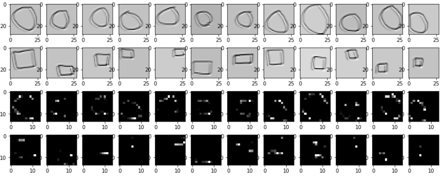
맨 윗 회색 두 줄은 conv 연산 출력 결과이고, 아래 검은색 두 줄은 maxpooling 연산 결과이다. conv 연산 결과만 보면 잘 모르겠는데 max pooling 연산을 보면 최댓값을 잘 이끌어내지 못하는 모습을 알 수 있다.
사실 conv 연산에 결과에서도 알 수 있는데 흰색 부분을 보면 된다.(잘 안보이긴 해요...) 흰색 부분이 많다는 것은 물체의 모양 특징을 필터가 잡아서 큰 값으로 출력했다는 뜻인데 도형 주변에 흰색이 거의 없고 두드러지지 않는다. 때문에 max pooling을 하게 되면 흰색 값이 적기 때문에 잘 출력되지 않는 것이다.
4. 역전파 구현하기(★★★★★)
제일 중요한 역전파 구현하기다. 이전 시간에 그렸던 그림과 함께 어떻게 코드로 구현했는지 관찰해 보자.
여기에 나오는 수학식들은 Numpy 딥러닝 시리즈를 정주행했다면 이해할 수 있다.
쉽게 이해하기 위해, 모니터를 2개 띄우고 그림과 코드를 서로 나란하게 보면서 본다면 금방 이해할 수 있다.
1) Wf, Bf 구하기

2) Wc, Bc 구하기
(1) Wc 구하기


위의 Wc 과정에서 ⑨번까지 동일하다.
# ⑨ 에서 sum을 통해 Bc의 shape 맞추기, dconv_dBc는 연산 불필요.
dL_dBc = np.reshape(np.sum(dL_dconv_s), (1, 1)) # (1, 1)
5. 훈련 및 결과 확인하기
1) 셔플 구현하기
train_X에 대한 라벨 train_Y를 짝 맞게 서로 잘 섞어서 훈련하면 더 좋은 성능을 낼 수 있다.
(참고: https://hiuaa.tistory.com/97, https://play.pixelblaster.ro/blog/2017/01/20/how-to-shuffle-two-arrays-to-the-same-order/ )

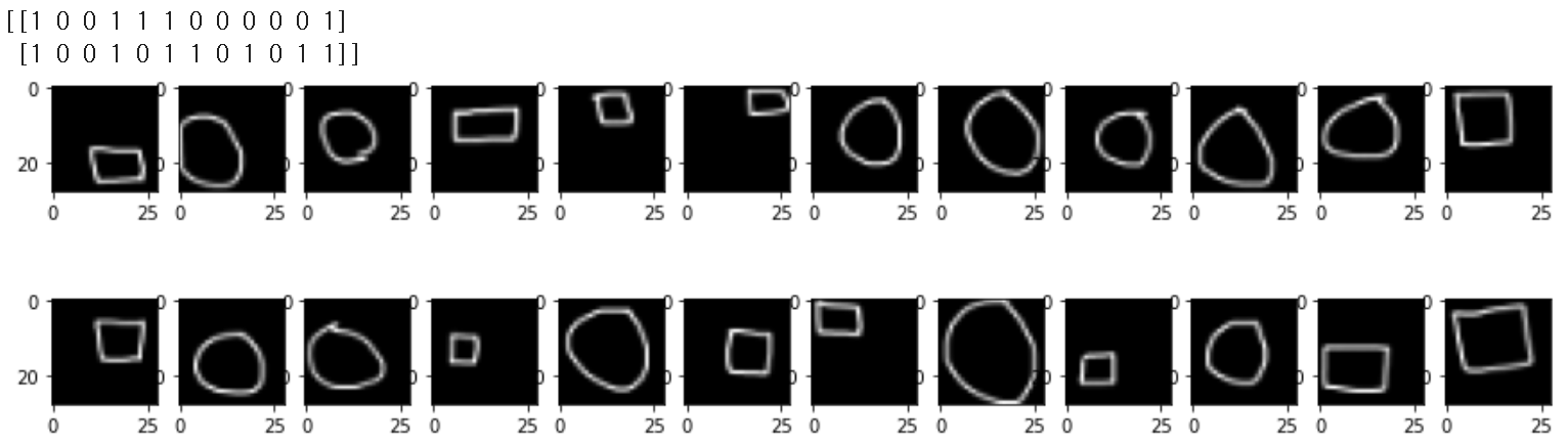
잘 섞인 것을 볼 수 있다.
2) 경사하강법 적용하기

3) 결과 확인하기

목표대로 훈련이 잘 성공한 듯 하다.
4) ★★★★★ 테스트 결과 확인하기

뭔가 하나도 맞지 않는다!!! 어찌된 일인가? 과적합 되었다는 뜻이다.
5) 훈련된 필터로 Conv2D, Max pooling 출력 결과 확인하기
테스트 데이터 적중률은 매우 좋지 않다. 왜 그런지 직접 살펴보자.

<훈련 전 Conv2D, Max pooling 출력>
<훈련 후 Conv2D, Max pooling 출력>

훈련 전과 훈련 후의 Conv2D를 비교하면, 흰색 윤곽이 뚜렷하게 나타난다. 이는 물체 모양 특징을 잘 파악했음을 의미한다. 그런데! Max pooling 결과 동그라미 모양인지, 네모 모양인지 잘 구별이 가지 않는다. 이는 데이터 부족, 필터 부족, 신경망 깊이 부족, 과적합 등 여러 가지 이유가 있다. 그래도 훈련 데이터는 잘 훈련되었다는 사실에 만족해도 좋다. (라이브러리 없이 Numpy 만으로 이정도면 잘 한 것이다!)
6. 번외, 원-세모 구별하기
코드를 그대로! 사용하고 원-네모 데이터에서 원-세모 데이터로 변경 후 훈련하여 보자.learning_rate = 0.015, epochs=700 으로 변경하여 오차율을 원-네모와 거의 일치시켰다.


훈련 결과가 원-네모 보다 원-세모가 훨씬 더 잘 일치한다. 그 이유를 아래 출력 결과에서 확인할 수 있다.
<훈련 전 Conv2D, Max pooling 출력>

<훈련 후 Conv2D, Max pooling 출력>

훈련 전과 훈련 후의 Conv2D를 비교하면, 훈련 전은 물체 모양 특징을 중구난방으로 추출한 느낌이나, 훈련 후는 대각선 성분을 잘 추출할 수 있도록 추상화 된 느낌이다.
이로써 Conv2D와 Max pooling을 어떻게 응용할 수 있는지 알아보았다. 아래는 전체 코드이다.
import numpy as np
import cv2
import matplotlib.pyplot as plt
train_X = []
train_path = '여러분의 경로/'
for i in range(24):
image_name = train_path + 'drawing' + '(' + str(i+1) + ')' + '.png'
image = cv2.imread(image_name, cv2.IMREAD_GRAYSCALE)
image = cv2.bitwise_not(image) # 검은색과 흰색을 반전하여 흰색은 1, 검은색은 0을 준다.
train_X.append(image)
train_X = np.array(train_X)*(10/255) # relu에서는 /255.0 안될듯
fig, ax = plt.subplots(2, 12, figsize=(15, 4))
for row in range(2):
for col in range(12):
ax[row][col].imshow(train_X[12*row+col], cmap='gray')
plt.show()
test_X = []
test_path = '/content/drive/MyDrive/Circle_Square_tiny/test/'
for i in range(4):
image_name = test_path + 'drawing' + '(' + str(i+1) + ')' + '.png'
image = cv2.imread(image_name, cv2.IMREAD_GRAYSCALE)
image = cv2.bitwise_not(image) # 검은색과 흰색을 반전하여 흰색은 1, 검은색은 0을 준다.
test_X.append(image)
test_X = np.array(test_X)*(10/255)
fig2, ax2 = plt.subplots(2, 2, figsize=(6, 3))
for row in range(2):
for col in range(2):
ax2[row][col].imshow(test_X[2*row+col], cmap='gray')
plt.show()
# circle → 0, square → 1
train_Y = np.concatenate((np.repeat(0, 12), np.repeat(1, 12)))
train_Y = np.reshape(train_Y, (1, -1))
train_Y = np.transpose(train_Y, (1, 0))
test_Y = np.concatenate((np.repeat(0, 2), np.repeat(1, 2)))
test_Y = np.reshape(test_Y, (1, -1))
test_Y = np.transpose(test_Y, (1, 0))
np.random.seed(230129)
Wc = np.random.randn(3, 3)
Bc = np.random.randn(1, 1)
Wf = np.random.randn(1, 196)
Bf = np.random.randn(1, 1)
conv_filter_size = 3
maxpooling_filter_size = 2
conv_stride = 1
maxpooling_stride = 2
conv_padding = 1
maxpooling_padding = 0 # -> 안씀
out_conv_size = 28 # 왜냐면 (28 - 3 + 2*1)/1 + 1 = 28 같은 크기로 출력됨.
out_maxpooling_size = 14 # 28/2 = 14
epsilon = 1e-4
def im2col(input, stride, padding, filter_size, output_size):
count = 0
input = np.pad(input, ((padding, padding), (padding, padding)))
for o_h in range(output_size):
for o_w in range(output_size):
a = input[stride*o_h : stride*o_h + filter_size, stride*o_w:stride*o_w + filter_size]
out = np.reshape(a, (1, -1))
if count == 0:
outs = out.copy()
else:
outs = np.concatenate((outs, out), axis=0)
count += 1
return np.transpose(outs, (1, 0))
def Conv2D(inputs, stride, padding, filter_size, output_size, weight, bias):
count = 0
for input in inputs:
im2col_input = im2col(input, stride, padding, filter_size, output_size)
conv = np.dot(weight.reshape(1, -1),im2col_input) + bias
conv = conv.reshape(output_size, output_size)
conv = conv[np.newaxis, :, :]
if count == 0:
outs = conv.copy()
else:
outs = np.concatenate((outs, conv))
count += 1
return outs
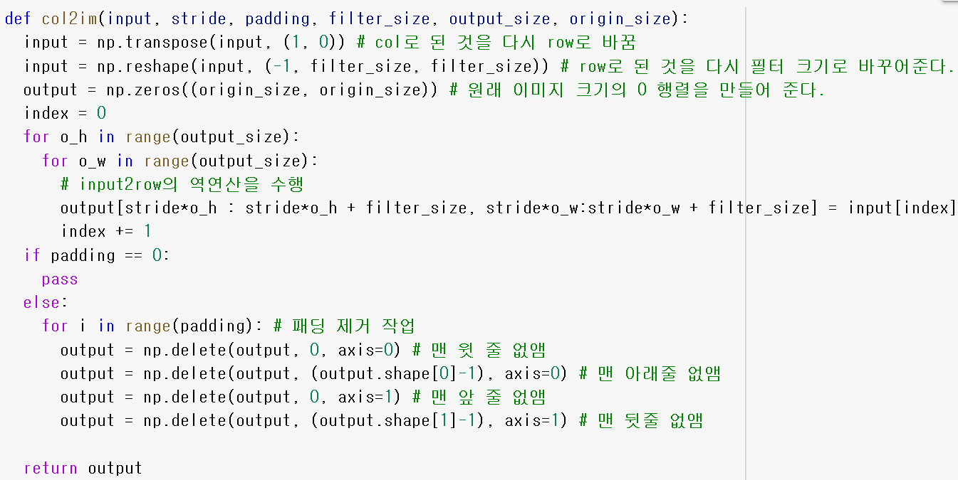
def col2im(input, stride, padding, filter_size, output_size, origin_size):
input = np.transpose(input, (1, 0)) # col로 된 것을 다시 row로 바꿈
input = np.reshape(input, (-1, filter_size, filter_size)) # row로 된 것을 다시 필터 크기로 바꾸어준다.
output = np.zeros((origin_size, origin_size)) # 원래 이미지 크기의 0 행렬을 만들어 준다.
index = 0
for o_h in range(output_size):
for o_w in range(output_size):
# input2row의 역연산을 수행
output[stride*o_h : stride*o_h + filter_size, stride*o_w:stride*o_w + filter_size] = input[index]
index += 1
if padding == 0:
pass
else:
for i in range(padding): # 패딩 제거 작업
output = np.delete(output, 0, axis=0) # 맨 윗 줄 없앰
output = np.delete(output, (output.shape[0]-1), axis=0) # 맨 아래줄 없앰
output = np.delete(output, 0, axis=1) # 맨 앞 줄 없앰
output = np.delete(output, (output.shape[1]-1), axis=1) # 맨 뒷줄 없앰
return output
def Max_Pooling(inputs, stride, filter_size, output_size):
count = 0
for input in inputs:
im2col_input = im2col(input, stride, 0, filter_size, output_size)
max_pooling = np.max(im2col_input, axis=0, keepdims=True)
max_pooling = np.reshape(max_pooling, (output_size, output_size))
out = max_pooling[np.newaxis, :, :]
if count == 0:
outs = out.copy()
else:
outs = np.concatenate((outs, out))
count += 1
return outs
def backward_Max_Pooling(inputs, origins, stride, filter_size, output_size, origin_size):
count = 0
for input, origin in zip(inputs, origins):
input = np.reshape(input, (1, -1))
repeat_max_pooling = np.tile(input, reps=[filter_size*filter_size, 1])
origin_im2col = im2col(origin, stride, 0, filter_size, output_size)
grad_max_pooling = np.where(input==origin_im2col, 1, 0)
grad_max_col2im = col2im(grad_max_pooling, stride, 0, filter_size, output_size, origin_size)
out = grad_max_col2im[np.newaxis, :, :]
if count == 0:
outs = out.copy()
else:
outs = np.concatenate((outs, out))
count += 1
return outs
# 순전파 정의
def forward (inputs, targets):
conv = Conv2D(inputs=inputs, stride=conv_stride, padding=conv_padding,
filter_size=conv_filter_size, output_size=out_conv_size,
weight=Wc, bias=Bc) # (batch, 28, 28)
relu = np.maximum(0, conv)
max_pooling = Max_Pooling(inputs=relu, stride=maxpooling_stride,
filter_size=maxpooling_filter_size,
output_size=out_maxpooling_size) # (batch, 14, 14)
flatten = np.reshape(max_pooling, (-1, out_maxpooling_size**2)) # (batch, 196)
fc = np.dot(Wf, np.transpose(flatten, (1, 0))) + Bf # (1, batch)
sigmoid = 1/(1+np.exp(-fc)) # (1, batch) → pred
targets = np.transpose(targets, (1, 0))
losses = np.sum(-targets*np.log1p(sigmoid) -
(1-targets)*np.log1p(1-(sigmoid))) # (1, batch)
return losses, sigmoid, fc, flatten, max_pooling, relu, conv
_, _, _, _, max_pooling, _, conv = forward(train_X, train_Y)
fig3, ax3 = plt.subplots(4, 12, figsize=(15, 6))
for row in range(4):
for col in range(12):
if row == 0 or row == 1:
ax3[row][col].imshow(conv[12*row+col], cmap='gray')
elif row == 2 or row == 3:
ax3[row][col].imshow(max_pooling[12*(row-2)+col], cmap='gray')
plt.show()
def loss_gradient(inputs, targets):
_, sigmoid, fc, flatten, max_pooling, relu, conv = forward(inputs, targets)
Y = np.transpose(targets, (1, 0)) # (1, batch)
dL_dsig = -1*( (Y / (sigmoid+epsilon)) - ( (1-Y) / (1-(sigmoid+epsilon)) ) ) # (1, batch)
dsig_dfc = ( 1/(1+np.exp(-fc)) ) * ( 1 - 1/(1+np.exp(-fc)) ) # (1, batch)
dL_dfc = dL_dsig * dsig_dfc # (1, batch)
# Wf, Bf 구하기
dfc_dWf = flatten # (batch, 14×14)
dL_dWf = np.dot(dL_dfc, dfc_dWf) # (1, 196)
dL_dBf = np.sum(dL_dfc, keepdims=True) # (1, 1)
dfc_dflatten = np.transpose(Wf, (1, 0)) # (196, 1)
dL_dflatten = np.transpose(np.dot(dfc_dflatten, dL_dfc), (1, 0))
# (196, batch) → (batch, 196)
"""flatten 연산은 max pooling 연산 결과를 shape 변형한 것에 불과,
따라서 dflatten_dmax는 dL_dflatten 값을 max pooling 출력 shape으로 바꾸는 것이다."""
dL_dmax = np.reshape(dL_dflatten, (-1, out_maxpooling_size, out_maxpooling_size))
# (batch, 14, 14)
"""max pooling의 출력을 되돌려 relu와 shape이 맞게 해 주어야 한다."""
dL_dmax = np.reshape(dL_dmax, (-1, 1, out_maxpooling_size**2)) # (batch, 1, 196)
"""batch 단위로 1행을 4행으로 복사하여 최대값 선택 전으로 되돌리기"""
dL_dmax = np.tile(dL_dmax, reps=[1, maxpooling_filter_size**2, 1]) # (batch, 4, 196)
"""column to image 연산을 통해 원래 이미지로 되돌리기"""
count = 0
for input in dL_dmax:
out = col2im(input=input, stride=maxpooling_stride, padding=0,
filter_size=maxpooling_filter_size,
output_size=out_maxpooling_size,
origin_size=out_conv_size) #out_conv_size = relu.shape[1]
out = out[np.newaxis, :, :]
if count == 0:
outs = out.copy()
else:
outs = np.concatenate((outs, out))
count += 1
dL_dmax = outs.copy() #(batch, 28, 28)
"""relu 이미지의 최대값은 1, 나머지는 0"""
dmax_drelu = backward_Max_Pooling(inputs=max_pooling, origins=relu,
stride=maxpooling_stride,
filter_size=maxpooling_filter_size,
output_size=out_maxpooling_size,
origin_size=out_conv_size) # 28에 패딩 1이면 30임
#(batch, 28, 28)
dL_drelu = dL_dmax * dmax_drelu # (batch, 28, 28)
"""cov 값에서 0보다 크면 1, 아니면 0"""
drelu_dconv = np.where(conv>=0, 1, 0) # (batch, 28, 28)
dL_dconv = dL_drelu * drelu_dconv # (batch, 28, 28)
dL_dconv_s = np.reshape(dL_dconv, (-1, 1, out_conv_size**2))
# (batch, 1, 28×28)
# Wc와 Bc를 구해보자
count = 0
for input in inputs:
dconv_dWc = im2col(input=input, stride=conv_stride, padding=conv_padding,
filter_size=conv_filter_size, output_size=out_conv_size)
dconv_dWc = dconv_dWc[np.newaxis, :, :]
if count == 0:
outs = dconv_dWc.copy()
else:
outs = np.concatenate((outs, dconv_dWc))
count += 1
dconv_dWc_s = np.transpose(outs, (0, 2, 1))
# (batch, 28, 28) -> (batch, 28×28, 9)
"""batch 단위의 행렬곱 실시"""
dL_dWc_sum = 0
for dL_dconv, dconv_dWc in zip(dL_dconv_s, dconv_dWc_s):
dL_dWc = np.dot(dL_dconv, dconv_dWc)
dL_dWc_sum += dL_dWc # (1, 9)
dL_dWc = np.reshape(dL_dWc_sum, (conv_filter_size, conv_filter_size)) # (3, 3)
dL_dBc = np.reshape(np.sum(dL_dconv_s), (1, 1)) # (1, 1)
return dL_dWf, dL_dBf, dL_dWc, dL_dBc
shuffle = np.arange(train_X.shape[0])
np.random.shuffle(shuffle)
train_X_shuffle = train_X[shuffle]
train_Y_shuffle = train_Y[shuffle]
print(np.reshape(train_Y_shuffle, (2, 12)))
fig4, ax4 = plt.subplots(2, 12, figsize=(15, 4))
for row in range(2):
for col in range(12):
ax4[row][col].imshow(train_X_shuffle[12*row+col], cmap='gray')
plt.show()
# 경사하강법 적용
learning_rate = 0.01
epochs = 500
for epoch in range(epochs+1):
shuffle = np.arange(train_X.shape[0])
np.random.shuffle(shuffle)
train_X_shuffle = train_X[shuffle]
train_Y_shuffle = train_Y[shuffle]
losses, pred, fc, flatten, max_pooling, relu, conv = forward(train_X_shuffle, train_Y_shuffle)
dL_dWf, dL_dBf, dL_dWc, dL_dBc = loss_gradient(train_X_shuffle, train_Y_shuffle)
Wf = Wf + -1*learning_rate*dL_dWf
Bf = Bf + -1*learning_rate*dL_dBf
Wc = Wc + -1*learning_rate*dL_dWc
Bc = Bc + -1*learning_rate*dL_dBc
if epoch % 50 == 0:
print('epoch :', epoch, '\n', 'loss :', losses, '\n',
'forward :' , '\n', pred, '\n', 'target :', '\n', np.reshape(train_Y_shuffle, (1, -1)))
_, pred, _, _, _, _, _ = forward(test_X, test_Y)
print('test pred :', pred)
print('test target : ', np.reshape(test_Y, (1, -1)))
_, _, _, _, max_pooling, relu, conv = forward(train_X, train_Y)
fig4, ax4 = plt.subplots(4, 12, figsize=(15, 6))
for row in range(4):
for col in range(12):
if row == 0 or row == 1:
ax4[row][col].imshow(conv[12*row+col], cmap='gray')
elif row == 2 or row == 3:
ax4[row][col].imshow(max_pooling[12*(row-2)+col], cmap='gray')
plt.show()'파이썬 프로그래밍 > Numpy 딥러닝' 카테고리의 다른 글
| 38.[RNN기초] 자연어 데이터는 어떻게 접근해야 할까? (0) | 2023.09.11 |
|---|---|
| 37. [CNN기초] 다채널(multi channel) 다루기 (0) | 2023.02.18 |
| 35. [CNN기초] 원, 네모를 구별하는 CNN 만들기(이론) (2) | 2023.01.28 |
| 34. [CNN기초] Max pooling, Average pooling 구현 (0) | 2023.01.26 |
| 33. [CNN기초] 이미지의 합성곱 훈련 -쉬운예제(실습)- (0) | 2023.01.21 |


