저번시간에 아래와 같이 3 × 3 이미지를 2 × 2 값으로 어떻게 훈련할 수 있는지 이야기하였다.
오늘은 이 내용을 코드로 작성해 보고자 한다.
예상하건데 필터는 1개이고, 선형분류기가 따로 없으므로 훈련 성과는 그리 좋을 것 같지 않다.

먼저 입력 Input과 목표 Target을 설정해 보자. numpy의 flipud와 fliplr을 이용하여 생성하면 편하다.
import numpy as np
import matplotlib.pyplot as plt
x_sorce1 = np.array([[0.1, 0.2, 0.3],
                     [0.4, 0.5, 0.6],
                     [0.7, 0.8, 0.9]])

x_sorce2 = np.flipud(x_sorce1) # sorce1의 좌우반전
x_sorce3 = np.fliplr(x_sorce1) # sorce1의 상하반전
x_sorce4 = np.fliplr(x_sorce2) # sorce2의 좌우반전


X = np.stack((x_sorce1, x_sorce2, x_sorce3, x_sorce4))

y_sorce1 = np.array([[0., 0.],
                     [0., 1.]])

y_sorce2 = np.flipud(y_sorce1) # sorce1의 좌우반전
y_sorce3 = np.fliplr(y_sorce1) # sorce1의 상하반전
y_sorce4 = np.fliplr(y_sorce2) # sorce2의 좌우반전

Y = np.stack((y_sorce1, y_sorce2, y_sorce3, y_sorce4))

fig, ax = plt.subplots(2, 4)
for x in range(4):
  ax[0][x].imshow(X[x], cmap='gray')
for y in range(4):
  ax[1][y].imshow(Y[y], cmap='gray')

print(X.shape)
print(Y.shape)
plt.show()
훈련에 필요한 변수들을 설정해 보자. 손코딩과 동일하게 하면 된다.
W = np.random.randn(2, 2)
B = np.random.randn(1, 1)

PADDING = 0
STRIDE = 1
FILTER_SIZE = W.shape[0] # 2

#여기서 X.shape은 (4, 3, 3,) (batch, width, height) 이므로
OUTPUT_SIZE = int((X.shape[1] - FILTER_SIZE + 2*PADDING)/STRIDE + 1) # 2
2차원 합성곱을 정의해 보자.
im2col 함수를 구현한 것인데 입력 Input에 대해 패딩을 실시 → 필터 크기로 슬라이싱 → image to row → image to colum을 실시한다.
def im2col(input, stride, padding, filter_size, output_size):
  count = 0
  input = np.pad(input, ((padding, padding), (padding, padding)))
  for o_h in range(output_size):
    for o_w in range(output_size):
      a = input[stride*o_h : stride*o_h + filter_size, stride*o_w:stride*o_w + filter_size]
      out = np.reshape(a, (1, -1))
      if count == 0:
        outs = out.copy()
      else:
        outs = np.concatenate((outs, out), axis=0)
      count += 1

  return np.transpose(outs, (1, 0))

im2col_image = im2col(input=X[0], stride=STRIDE, padding = PADDING, filter_size=FILTER_SIZE, output_size=OUTPUT_SIZE)
print(im2col_image)
합성곱 함수 정의이다. im2col 과 w의 선형 연산 → 출력 이미지 크기로 변환 → 쌓기를 하면 (batch, output height, output width)로 출력된다.
def Conv2D(inputs, stride, padding, filter_size, output_size, weight, bias):
  count = 0
  for input in inputs:
    im2col_input = im2col(input, stride, padding, filter_size, output_size)
    conv = np.dot(weight.reshape(1, -1),im2col_input) + bias
    conv = conv.reshape(output_size, output_size)
    conv = conv[np.newaxis, :, :]
    if count == 0:
      outs = conv.copy()
    else:
      outs = np.concatenate((outs, conv))
    count += 1
  return outs

print(Conv2D(inputs=X, stride=STRIDE, padding = PADDING,
             filter_size=FILTER_SIZE, output_size=OUTPUT_SIZE,
             weight=W, bias = B))
순전파(forward)를 정의해 보자.
Conv2D 출력이 모델의 예측값(pred)가 된다.
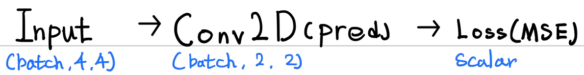
def forward(inputs, targets):
  pred = Conv2D(inputs=X, stride=STRIDE, padding = PADDING,
                filter_size=FILTER_SIZE, output_size=OUTPUT_SIZE,
                weight=W, bias = B)
  loss = np.mean(np.power((pred - targets), 2))
  return loss, pred

print(forward(X, Y))
역전파를 정의해 보자.

가장 구현해야 할 것은 dConv_dW인데, 이는 im2col 연산의 전치(Transpose)인 image to row 즉 im2row가 된다. 이를 구현할 함수이다. im2col 함수를 이용한 것인데 왜 따로 함수를 정의하면 im2col 함수는 Conv2D 함수에서 batch 단위 연산에 사용하기 위한 이미지 1개에 대한 연산이다. batch 로 쌓아야 하므로 함수를 만들어 주었다. 내부 안에 im2col 함수가 있음에 주목하자.
# im2col에 대한 역전파 함수를 만들어보자. .
# conv 연산에 대한 W의 기울기 => im2col의 전치임. image 2 row
# 이를 batch 단위로 묶자.
def grad_conv_W(inputs, stride, padding, filter_size, output_size):
  count = 0
  for input in inputs:
    input_to_col = im2col(input, stride, padding, filter_size, output_size)
    out = np.transpose(input_to_col, (1, 0)) # 전치시켜줘야 함. -> image to row
    out = out[np.newaxis, :, :]
    if count == 0:
      outs = out.copy()
    else:
      outs = np.concatenate((outs, out))
    count += 1
  return outs

back_input = grad_conv_W(inputs=X, stride=STRIDE, padding = PADDING,
                         filter_size=FILTER_SIZE, output_size=OUTPUT_SIZE)
print(back_input)
im2row와 출력 부분 계산 결과와 선형 연산을 해야 한다. batch번 실행하고 누적해야 하므로(왜냐면 가중치 W는 이미지마다 연산되었으므로, 역전파 과정에서는 다 더해야 한다.) 따로 함수를 지정해 주었다.
# batch 단위(index로 번호 부여)로 하나씩 계산하고 다 더함
# out은 출력, cal은 계산(W*X + B), W는 가중치이다.
# batch 개수의 dout_dW가 계산될 텐데 같은 가중치에 의해 계산되었으므로
# 그냥 더해준다.
def grad_loss_W(dout_dcal, dcal_dW):
  dout_dW_sum = 0
  for index in range(dout_dcal.shape[0]):
    dout_dW = np.dot(np.reshape(dout_dcal[index], (1, -1)), dcal_dW[index])
    dout_dW_sum += dout_dW
  return dout_dW_sum
아래는 전체 역전파 코드이다.
# 역전파를 해 보자. 간단하다 행렬곱 생각을 하면 된다.
def loss_gradient(input, target, pred):
  dL_dY = 2*(pred - target) # (batch, 2, 2)
  #print('dL_dY :', dL_dY)

  # W(1, 4)와 im2col(4, 4)의 행렬 연산은 (1, 4)임. 따라서 이에 맞게 변환하여야 한다.
  dL_dY = np.reshape(dL_dY, (-1, 4))  # (batch, 2, 2) -> (batch, 4)
  #print(dL_dY)

  dY_dW = grad_conv_W(inputs=X, stride=STRIDE, padding = PADDING,
                      filter_size=FILTER_SIZE, output_size=OUTPUT_SIZE) # (batch, 4, 4)
  #print(dY_dW)

  dL_dW = grad_loss_W(dL_dY, dY_dW) # (1, 4)
  #print(dL_dW)

  dL_dW = dL_dW.reshape(FILTER_SIZE, FILTER_SIZE) # (2, 2)
  #print('dL_dW :', dL_dW)

  dL_dB = np.sum(dL_dY, keepdims=True)
  #print('dL_dB', dL_dB)

  return dL_dW, dL_dB

loss, conv = forward(X, Y)
print(loss_gradient(X, Y, conv))
경사하강법을 적용하여 훈련해 보자.
# 경사하강법 적용
learning_rate = 0.001
epochs = 1000
for epoch in range(epochs+1):
  _, predict = forward(X, Y)

  dL_dW, dL_dB = loss_gradient(X, Y, predict)

  W = W + -1*learning_rate*dL_dW
  B = B + -1*learning_rate*dL_dB

  if epoch % 100 == 0:
    print('epoch :', epoch, '\n', 'forward :' , '\n', predict)
훈련 결과가 썩 좋지 못하다. 1000회 훈련했다면 노란색 부분이 1, 나머지는 0에 가까워야 한다. 이전 예제에서도 알 수 있듯이 분류기를 넣지 않은 것이 크다. 이미지를 그려 가며 확인해 보자.
fig2, ax2 = plt.subplots(2, 4)
_, predict = forward(X, Y)
for y in range(4):
  ax2[0][y].imshow(Y[y], cmap='gray')
for pred in range(4):
  ax2[1][pred].imshow(predict[pred], cmap='gray')
plt.show()

아래는 전체 코드이다.
import numpy as np
import matplotlib.pyplot as plt
x_sorce1 = np.array([[0.1, 0.2, 0.3],
                     [0.4, 0.5, 0.6],
                     [0.7, 0.8, 0.9]])

x_sorce2 = np.flipud(x_sorce1) # sorce1의 좌우반전
x_sorce3 = np.fliplr(x_sorce1) # sorce1의 상하반전
x_sorce4 = np.fliplr(x_sorce2) # sorce2의 좌우반전


X = np.stack((x_sorce1, x_sorce2, x_sorce3, x_sorce4))

y_sorce1 = np.array([[0., 0.],
                     [0., 1.]])

y_sorce2 = np.flipud(y_sorce1) # sorce1의 좌우반전
y_sorce3 = np.fliplr(y_sorce1) # sorce1의 상하반전
y_sorce4 = np.fliplr(y_sorce2) # sorce2의 좌우반전

Y = np.stack((y_sorce1, y_sorce2, y_sorce3, y_sorce4))

fig, ax = plt.subplots(2, 4)
for x in range(4):
  ax[0][x].imshow(X[x], cmap='gray')
for y in range(4):
  ax[1][y].imshow(Y[y], cmap='gray')
plt.show()

W = np.random.randn(2, 2)
B = np.random.randn(1, 1)

PADDING = 0
STRIDE = 1
FILTER_SIZE = W.shape[0] # 2

#여기서 X.shape은 (4, 3, 3,) (batch, width, height) 이므로
OUTPUT_SIZE = int((X.shape[1] - FILTER_SIZE + 2*PADDING)/STRIDE + 1) # 2

def im2col(input, stride, padding, filter_size, output_size):
  count = 0
  input = np.pad(input, ((padding, padding), (padding, padding)))
  for o_h in range(output_size):
    for o_w in range(output_size):
      a = input[stride*o_h : stride*o_h + filter_size, stride*o_w:stride*o_w + filter_size]
      out = np.reshape(a, (1, -1))
      if count == 0:
        outs = out.copy()
      else:
        outs = np.concatenate((outs, out), axis=0)
      count += 1

  return np.transpose(outs, (1, 0))

def Conv2D(inputs, stride, padding, filter_size, output_size, weight, bias):
  count = 0
  for input in inputs:
    im2col_input = im2col(input, stride, padding, filter_size, output_size)
    conv = np.dot(weight.reshape(1, -1),im2col_input) + bias
    conv = conv.reshape(output_size, output_size)
    conv = conv[np.newaxis, :, :]
    if count == 0:
      outs = conv.copy()
    else:
      outs = np.concatenate((outs, conv))
    count += 1
  return outs

def forward(inputs, targets):
  pred = Conv2D(inputs=X, stride=STRIDE, padding = PADDING,
                filter_size=FILTER_SIZE, output_size=OUTPUT_SIZE,
                weight=W, bias = B)
  loss = np.mean(np.power((pred - targets), 2))
  return loss, pred

# im2col에 대한 역전파 함수를 만들어보자. .
# conv 연산에 대한 W의 기울기 => im2col의 전치임. image 2 row
# 이를 batch 단위로 묶자.
def grad_conv_W(inputs, stride, padding, filter_size, output_size):
  count = 0
  for input in inputs:
    input_to_col = im2col(input, stride, padding, filter_size, output_size)
    out = np.transpose(input_to_col, (1, 0)) # 전치시켜줘야 함. -> image to row
    out = out[np.newaxis, :, :]
    if count == 0:
      outs = out.copy()
    else:
      outs = np.concatenate((outs, out))
    count += 1
  return outs

# batch 단위(index로 번호 부여)로 하나씩 계산하고 다 더함
# out은 출력, cal은 계산(W*X + B), W는 가중치이다.
# batch 개수의 dout_dW가 계산될 텐데 같은 가중치에 의해 계산되었으므로
# 그냥 더해준다.
def grad_loss_W(dout_dcal, dcal_dW):
  dout_dW_sum = 0
  for index in range(dout_dcal.shape[0]):
    dout_dW = np.dot(np.reshape(dout_dcal[index], (1, -1)), dcal_dW[index])
    dout_dW_sum += dout_dW
  return dout_dW_sum

# 역전파를 해 보자. 간단하다 행렬곱 생각을 하면 된다.
def loss_gradient(input, target, pred):
  dL_dY = 2*(pred - target) # (batch, 2, 2)
  #print('dL_dY :', dL_dY)

  # W(1, 4)와 im2col(4, 4)의 행렬 연산은 (1, 4)임. 따라서 이에 맞게 변환하여야 한다.
  dL_dY = np.reshape(dL_dY, (-1, 4))  # (batch, 2, 2) -> (batch, 4)
  #print(dL_dY)

  dY_dW = grad_conv_W(inputs=X, stride=STRIDE, padding = PADDING,
                      filter_size=FILTER_SIZE, output_size=OUTPUT_SIZE) # (batch, 4, 4)
  #print(dY_dW)

  dL_dW = grad_loss_W(dL_dY, dY_dW) # (1, 4)
  #print(dL_dW)

  dL_dW = dL_dW.reshape(FILTER_SIZE, FILTER_SIZE) # (2, 2)
  #print('dL_dW :', dL_dW)

  dL_dB = np.sum(dL_dY, keepdims=True)
  #print('dL_dB', dL_dB)

  return dL_dW, dL_dB

# 경사하강법 적용
learning_rate = 0.001
epochs = 1000
for epoch in range(epochs+1):
  _, predict = forward(X, Y)

  dL_dW, dL_dB = loss_gradient(X, Y, predict)

  W = W + -1*learning_rate*dL_dW
  B = B + -1*learning_rate*dL_dB

  if epoch % 100 == 0:
    print('epoch :', epoch, '\n', 'forward :' , '\n', predict)

fig2, ax2 = plt.subplots(2, 4)
_, predict = forward(X, Y)
for y in range(4):
  ax2[0][y].imshow(Y[y], cmap='gray')
for pred in range(4):
  ax2[1][pred].imshow(predict[pred], cmap='gray')
plt.show()'파이썬 프로그래밍 > Numpy 딥러닝' 카테고리의 다른 글
| 35. [CNN기초] 원, 네모를 구별하는 CNN 만들기(이론) (2) | 2023.01.28 |
|---|---|
| 34. [CNN기초] Max pooling, Average pooling 구현 (0) | 2023.01.26 |
| 32. [CNN기초] 이미지의 합성곱 훈련 -쉬운예제(이론)- (0) | 2023.01.20 |
| 31. [CNN기초] 2차원 배열 합성곱 - image to column-2 (0) | 2023.01.11 |
| 30. [CNN기초] 2차원 배열 합성곱 - image to column 구현 (0) | 2023.01.06 |


