일반적으로 도함수의 정의는 아래와 같다.
이를 파이썬 코드로 표현해 보자
def deriv(func, input, delta=0.001):
    return (func(input + delta) - func(input)) / delta
delta는 \(\Delta x\)의 표현으로 값을 줄리면 더 정확한 도함수를 얻겠지만...
연산이 많은 작업이라면 오래 걸릴 수 있으므로 적당히 하는 것을 추천
이차함수 \(x^{2}\) 와 도함수를 그래프로 그려보자.
import numpy as np
import matplotlib.pyplot as plt

def square(x):
    return np.power(x,2)

def deriv(func, input, delta=0.001):
    return (func(input + delta) - func(input)) / delta

x = np.arange(-2, 2, 0.01)
plt.plot(x, square(x), 'r', label='square')
plt.plot(x, deriv(square, x), 'b', label='deriv_square')
plt.legend()
plt.grid(True)
plt.show()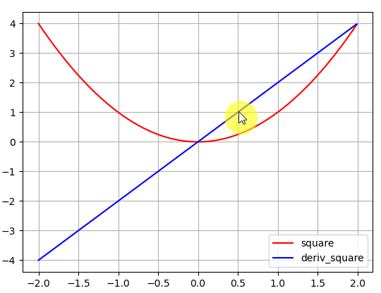
그래프에서 빨간 그래프는 \(x^{2}\) 함수의 그래프이고 파란 그래프는 \(x^{2}\)의 도함수 \(2x\)의 그래프이다.
x가 0.5일 때 도함수 값이 1을 가리키므로 잘 표현된 것을 알 수 있다.
함성함수의 도함수를 구하여 보자.
먼저 \(f_{2}(x) = x^{2}\), \(f_{1}(x) = 2x\)로 정의하자.
이에 대한 합성함수 \(h(x) = f_{2}(f_{1}(x))\)로 표현할 수 있고
체인 룰 \(\frac{dy}{dx} = \frac{dy}{du} \frac{du}{dx}\)을 이용하면
\(h^{'}(x) = \frac{d}{df_{1}(x)}f_{2}(f_{1}(x)) \times \frac{d}{dx}f_{1}(x)\)로 표현할 수 있다.
이를 파이썬 코드로 표현해 보면
(reference : https://github.com/flourscent/DLFS_code/blob/master/01_foundations/Code.ipynb)
def chain_deriv_2(chain, input):
    f1 = chain[0]
    f2 = chain[1]

    # f1(x)
    f1_x = f1(input)

    # d(f1(x))/dx
    df1_dx = deriv(f1, input)

    # d(f2(x))/d(f1(x))
    df2_df1 = deriv(f2, f1_x)

    # d(f2(f1(x))) / dx =  d(f2(x))/d(f1(x)) * d(f1(x))/dx
    return df2_df1 * df1_dx
제대로 동작하는지 확인해 볼 차례다.
\(h(x) = f_{2}(f_{1}(x)) = (2x)^{2}\) 이고
\(h^{'}(x) = \frac{d}{df_{1}(x)}f_{2}(f_{1}(x)) \times \frac{d}{dx}f_{1}(x) = 2(2x) \times 2 = 8x\)이므로
이를 그래프로 그려보고 맞는지 확인해 볼 수 있다.
파이썬 코드를 보자.
import numpy as np
import matplotlib.pyplot as plt

def linear(x):
    return 2*x

def square(x):
    return np.power(x,2)

def deriv(func, input, delta=0.001):
    return (func(input + delta) - func(input)) / delta

def comp_func(list_func, x):
    f1 = list_func[0]
    f2 = list_func[1]
    return f2(f1(x))

def chain_deriv_2(chain, input):
    f1 = chain[0]
    f2 = chain[1]

    # f1(x)
    f1_x = f1(input)

    # d(f1(x))/dx
    df1_dx = deriv(f1, input)

    # d(f2(x))/d(f1(x))
    df2_df1 = deriv(f2, f1_x)

    # d(f2(f1(x))) / dx =  d(f2(x))/d(f1(x)) * d(f1(x))/dx
    return df2_df1 * df1_dx

func_list = [linear, square]

x = np.arange(-2, 2, 0.01)
plt.plot(x, comp_func(func_list, x), 'r', label='comp_func')
plt.plot(x, chain_deriv_2(func_list, x), 'b', label='chain_deriv_2')
plt.legend()
plt.grid(True)
plt.show()
이를 출력해 본 것이다.
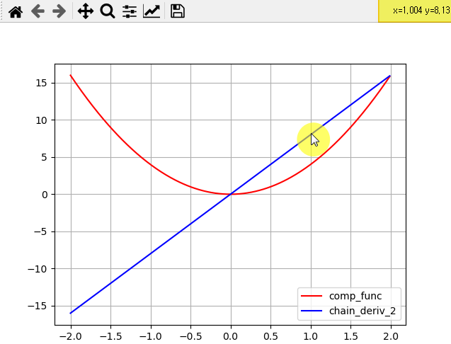
빨간색 그래프는 합성함수, 파란색 그래프는 합성함수의 도함수이다.
x=1인 지점에서 y값은 약 8.13을 가리키므로 잘 맞는다는 것을 알 수 있다.
'파이썬 프로그래밍 > 딥러닝과 수학' 카테고리의 다른 글
| 6. 2차원 행렬을 입력받는 합성함수의 도함수(이론) (0) | 2021.12.31 |
|---|---|
| 5. 벡터 합성함수의 도함수 표현 (0) | 2021.12.29 |
| 4. 벡터 입력에 대한 합성함수 표현 (0) | 2021.12.29 |
| 3. 입력이 여러 개인 함수와 도함수의 표현 (0) | 2021.12.28 |
| 1. 함수와 합성함수의 표현 (0) | 2021.12.27 |


