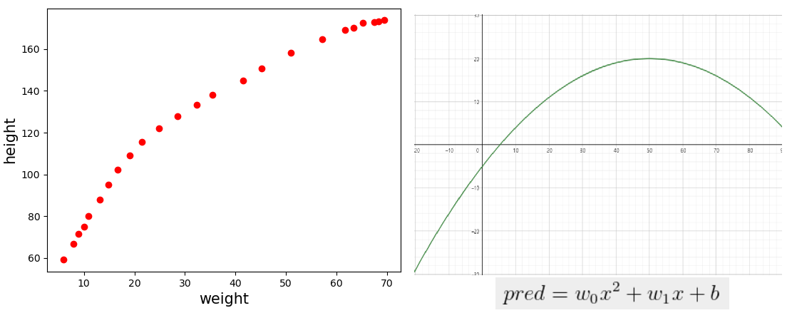
저번 차시에서 단층 퍼셉트론으로는 XOR 문제를 해결할 수 없다는 것을 알았다. 이번엔 실제로 와 닫는 문제를 가져왔다. 이번 목표는 단층 퍼셉트론으로 몸무게에 따른 키를 예측하는 모델을 만들어 보자.

몸무게와 키는 대략적으로 비례하는 것을 다들 알고 있을 것이다. 아기를 키워보면 알게되는 사실이 있는데 몸무게와 키가 정비례하는 것처럼 쭉쭉 큰다는 것이다. 그러다가 성장기가 지나면 키는 성장이 멈추지만 몸무게는 몸이 허락하는 한 한계가 없다(...) 이런 관계를 단층 퍼셉트론으로 모델을 만들 수 있을까?
1. 데이터 준비 및 확인
위의 파일을 임포트 하고 입력값, 목표값 등을 나누고 그래프를 그려보자
import numpy as np
import matplotlib.pyplot as plt
from numpy import genfromtxt


np.random.seed(220112)

data = genfromtxt('weight_height.csv', delimiter=',', skip_header=1)
input = data[:, 0]
target = data[:, 1]

input = input.reshape(-1, 1)
target = target.reshape(-1, 1)

plt.plot(input, target, 'ro')
plt.xlabel('weight', size=15)
plt.ylabel('height', size=15)
plt.show()
2. pred = wx +b의 선형회귀식
이 식을 단층 퍼셉트론 중 하나인 선형회귀식으로 표현할 수 있을까? pred = X*W + B 모델로 만들어 보겠다. 전체 코드이다. 구현에 대해서는 (https://toyourlight.tistory.com/12) 여기를 참고하길 바란다.
import numpy as np
import matplotlib.pyplot as plt
from numpy import genfromtxt


np.random.seed(220112)

data = genfromtxt('weight_height.csv', delimiter=',', skip_header=1)
input = data[:, 0] * 0.1 # np.power 연산에서 overflow 방지
target = data[:, 1] * 0.1 # np.power 연산에서 overflow 방지

input = input.reshape(-1, 1)
target = target.reshape(-1, 1)

W = np.random.randn(1, 1)
B = np.random.randn(1, 1)

learning_rate = 0.001

def linear_forward(X, Y, W, B):
    pred = np.dot(X, W) + B
    loss = np.mean(np.power(Y - pred, 2))

    return pred, loss

def loss_gradient(X, Y, W, B):
    XWB = np.dot(X, W) + B
    dL_dg = 2*(XWB - Y)
    dg_dW = np.transpose(X, (1, 0))
    dL_dW = np.dot(dg_dW, dL_dg)
    dL_dB = np.sum(dL_dg, axis=0)
    return dL_dW, dL_dB

_, loss = linear_forward(input, target, W, B)
print('loss : ', loss)


for i in range(100):
    dL_dW, dL_dB = loss_gradient(input, target, W, B)
    W = W + -1*learning_rate * dL_dW
    B = B + -1*learning_rate * dL_dB

pred, loss = linear_forward(input, target, W, B)
print('loss : ', loss)
print('W : ', W)
print('B : ', B)

plt.plot(input, target, 'ro', label='target')
plt.plot(input, pred, 'b', label='pred')
plt.xlabel('weight', size=15)
plt.ylabel('height', size=15)
plt.legend()
plt.show()
결과 확인
loss : 30.267319253924295
loss : 1.626183134825925
W : 2.00994212
B : 5.15076958
파란색 선은 몸무게가 x일 때 pred = 2.00*x + 5.15 로 키를 예측하는 선형회귀식을 표현한 것이다.
목표값은 완만한 곡선 형태를 띄는데 우리의 모델인 pred는 직선 형태이므로 잘 예측하지 못할 것 같다.
3. pred = w_0x^{2} + w_1x + b 의 선형회귀식
목표값을 보아하니 2차 방정식과 좀 비슷하지 않을까? 생각해 볼 수 있다. 즉, 모델인 선형회귀식을
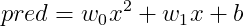
형태로 예측할 수 있지 않을까? 그러면 좀 더 정확해 지려나? 한번 해 보자. 이를 구현한 아이디어를 코드로 표현해 보았다.
input2 = np.hstack((np.power(input, 2), input))

W2 = np.random.randn(2, 1)
B2 = np.random.randn(1, 1)

learning_rate2 = 0.00005

pred2, loss2 = linear_forward(input2, target, W2, B2)

for i in range(100):
    dL_dW, dL_dB = loss_gradient(input2, target, W2, B2)
    W2 = W2 + -1*learning_rate2 * dL_dW
    B2 = B2 + -1*learning_rate2 * dL_dB
input2 = [x^(2), x] 로 표현하기 위해 np.hstack을 사용하였다.
입력 특성이 2개이므로 weight의 shape는 당연히 (2, 1)이여야 한다.
학습률을 설정한다. 왜 이렇게 작냐고 하면 x^(2) 이므로 학습을 천천히 시켜야 한다.
이 값으로 forward 연산, backward 연산과 훈련을 실시한다. 아래는 전체코드와 결과이다. 어떻게 되었을까?
import numpy as np
import matplotlib.pyplot as plt
from numpy import genfromtxt


np.random.seed(220112)

data = genfromtxt('weight_height.csv', delimiter=',', skip_header=1)
input = data[:, 0] * 0.1 # np.power 연산에서 overflow 방지
target = data[:, 1] * 0.1 # np.power 연산에서 overflow 방지

input = input.reshape(-1, 1)
input2 = np.hstack((np.power(input, 2), input))
target = target.reshape(-1, 1)

W = np.random.randn(1, 1)
B = np.random.randn(1, 1)

W2 = np.random.randn(2, 1)
B2 = np.random.randn(1, 1)

learning_rate = 0.001
learning_rate2 = 0.00005

def linear_forward(X, Y, W, B):
    pred = np.dot(X, W) + B
    loss = np.mean(np.power(Y - pred, 2))

    return pred, loss

def loss_gradient(X, Y, W, B):
    XWB = np.dot(X, W) + B
    dL_dg = 2*(XWB - Y)
    dg_dW = np.transpose(X, (1, 0))
    dL_dW = np.dot(dg_dW, dL_dg)
    dL_dB = np.sum(dL_dg, axis=0)
    return dL_dW, dL_dB

pred, loss = linear_forward(input, target, W, B)
pred2, loss2 = linear_forward(input2, target, W2, B2)
print('loss : ', loss2)

for i in range(100):
    dL_dW, dL_dB = loss_gradient(input, target, W, B)
    W = W + -1*learning_rate * dL_dW
    B = B + -1*learning_rate * dL_dB

for i in range(100):
    dL_dW, dL_dB = loss_gradient(input2, target, W2, B2)
    W2 = W2 + -1*learning_rate2 * dL_dW
    B2 = B2 + -1*learning_rate2 * dL_dB

pred, loss = linear_forward(input, target, W, B)
pred2, loss2 = linear_forward(input2, target, W2, B2)
print('loss : ', loss2)


print('W2 : ', W2)
print('B2 : ', B2)

plt.plot(input, target, 'ro', label='target')
plt.plot(input, pred, 'b', label='pred')
plt.plot(input, pred2, 'g', label='pred2')
plt.xlabel('weight', size=15)
plt.ylabel('height', size=15)
plt.legend()
plt.show()
loss : 1902.0074420334786
loss : 18.148144748416307
W2 : [[0.29567561]
[0.56796051]]
B2 : [[2.71944333]]
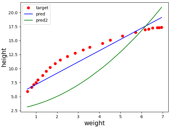
오차가 더 심해진것 같다(...) 차라리 일차 선형회귀식이 더 나은 것 같기도 하다.
4. 선형회귀식의 문제점
일단 선형회귀식의 정의부터 알아야겠지? 엄밀한 수학적 정의부터 보자.
선형회귀식은 계수가 선형결합을 만족하는 방정식이다. 구체적으로 다음과 같다.
1) 계수는 weight과 bias를 말한다. (입력값 x가 아니다! 이거 은근히 헷갈리던데...)
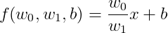
2) 선형결합이란 다음 두 조건을 만족한다. f가 weight 의 함수일 때

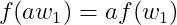
예를 들어 보자. f(w, b) = wx + b의 함수가 있을 때
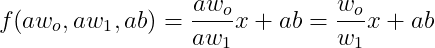
(1) 첫 번째 규칙 : 성립한다.


(2) 두 번째 규칙 : 성립한다.

아래의 방정식은 입력에 대해 2차 방정식이지만 계수에 대해서는 1차 방정식이다. 위의 선형결합이 성립한다. 궁금하면 직접 해 보자

선형회귀식은 굉장히 단순한 식이고, 선형회귀가 아닌 방정식도 많다. 예를 들어 아래의 식은 선형회귀식일까?
선형회귀식 조건을 확인해 보자

성립되지 않는다.
5. 결론
선형회귀식으로 이루어진 단층퍼셉트론은 데이터가 복잡해질 수록 학습이 잘 되지 않는다.
다음시간에는 XOR 문제를 어떻게 해결했는지 알아보자.
'파이썬 프로그래밍 > Numpy 딥러닝' 카테고리의 다른 글
| 14. 다층 퍼셉트론(MLP) 등장 - 1.XOR 문제 해결(심화이론) (0) | 2022.01.19 |
|---|---|
| 13. 다층 퍼셉트론(MPL) 등장 - 1.XOR 문제 해결(기초이론) (0) | 2022.01.18 |
| 11. 단층 퍼셉트론의 한계-1.XOR 문제 (0) | 2022.01.11 |
| 10. 단층 퍼셉트론 (0) | 2022.01.10 |
| 9. 다중 분류 구현하기(심화실습) (2) | 2022.01.09 |


